Energy-Flow Cosmology (EFC)

1. Frontmatter

This document is the canonical master specification for Energy-Flow Cosmology (EFC). It defines the formal structure and relations between:

• EFC-S: structural and halo-level descriptions,
• EFC-D: energy-flow dynamics on top of these structures,
• EFC-C₀: base mapping between entropy and information capacity.

The goal is a compact, mathematically explicit core that higher-level models, simulations and epistemic layers can reference without ambiguity.

Version history

• v1.0 Initial formal master specification (structure, fields, schematic figures).
• v1.1 Layout polish, improved spacing, figure placement, and explicit DOI frontmatter.

2. Overview

EFC treats the universe as a thermodynamic information system driven by gradients in energy flow and entropy. Instead of adding invisible components, the model starts from:

• energy distribution,
• entropy gradients,
• information capacity.

The three base layers are:

• EFC-S defines how low-entropy matter distributions organise into halo-like structures,
• EFC-D defines how local energy-flow potentials and their gradients shape dynamics,
• EFC-C₀ defines how entropy and structure map to information capacity and cognitive potential.

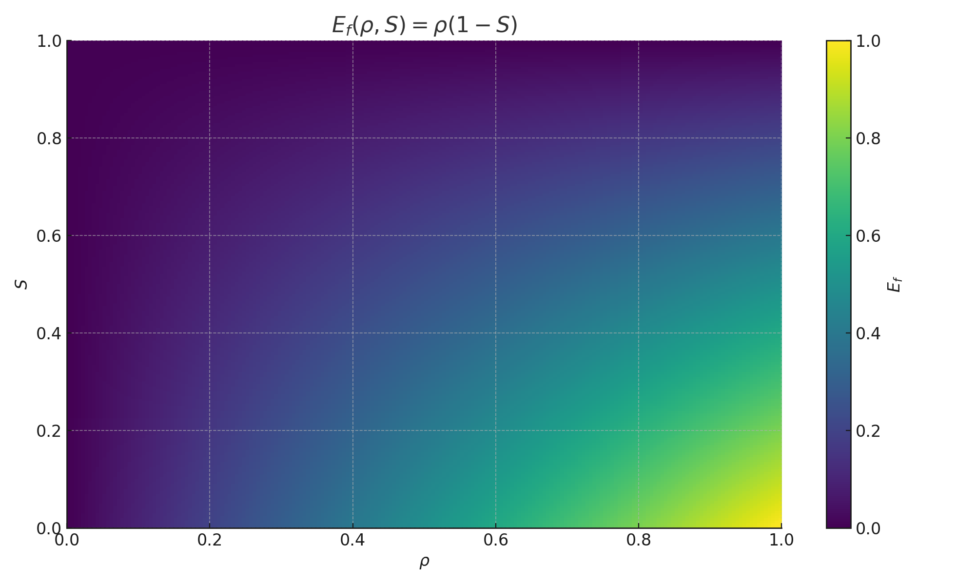
A central object is the local energy-flow potential:

which couples density and entropy into a single field.

3. Illustrative Field and Profiles

This section collects schematic figures that visualise the basic EFC fields and profiles. They are theoretical examples consistent with the definitions in the later sections.

3.1 Energy-flow potential field $E_f(\rho ,S)$

Figure 1 shows a schematic map of the energy-flow potential $E_f(\rho ,S)=\rho (1-S)$ over the $(\rho ,S)$ plane.

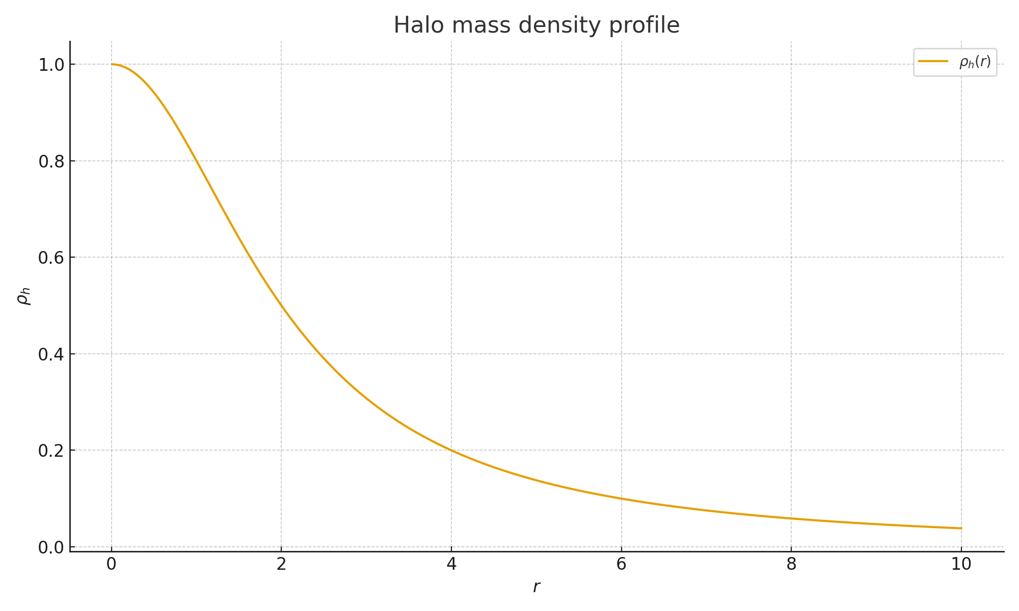
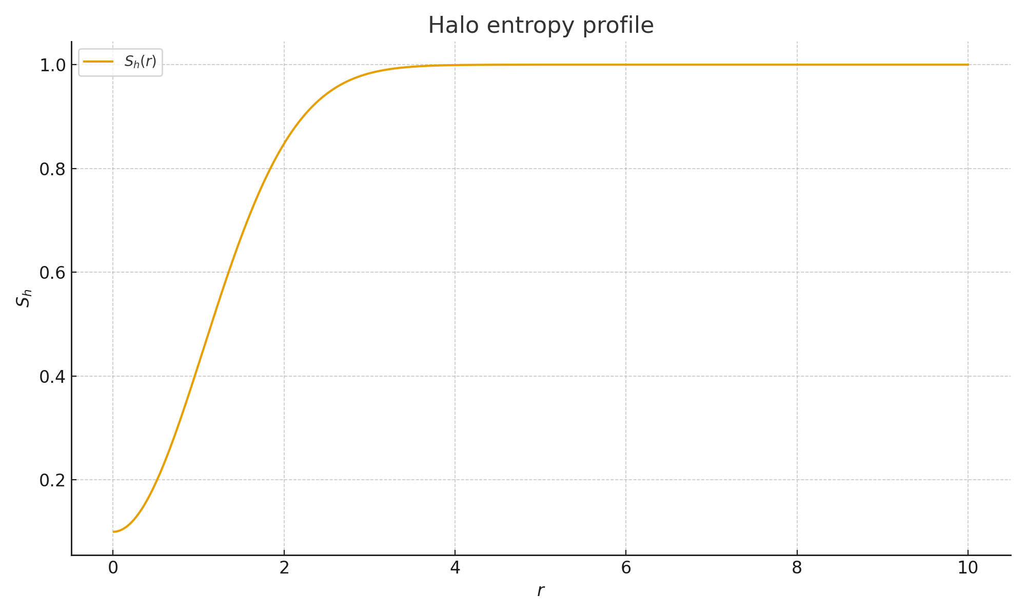
3.2 Halo profiles: mass and entropy

EFC-S models halos as joint profiles in mass density and entropy, ${\rho }_h(r)$ and $S_h(r)$.

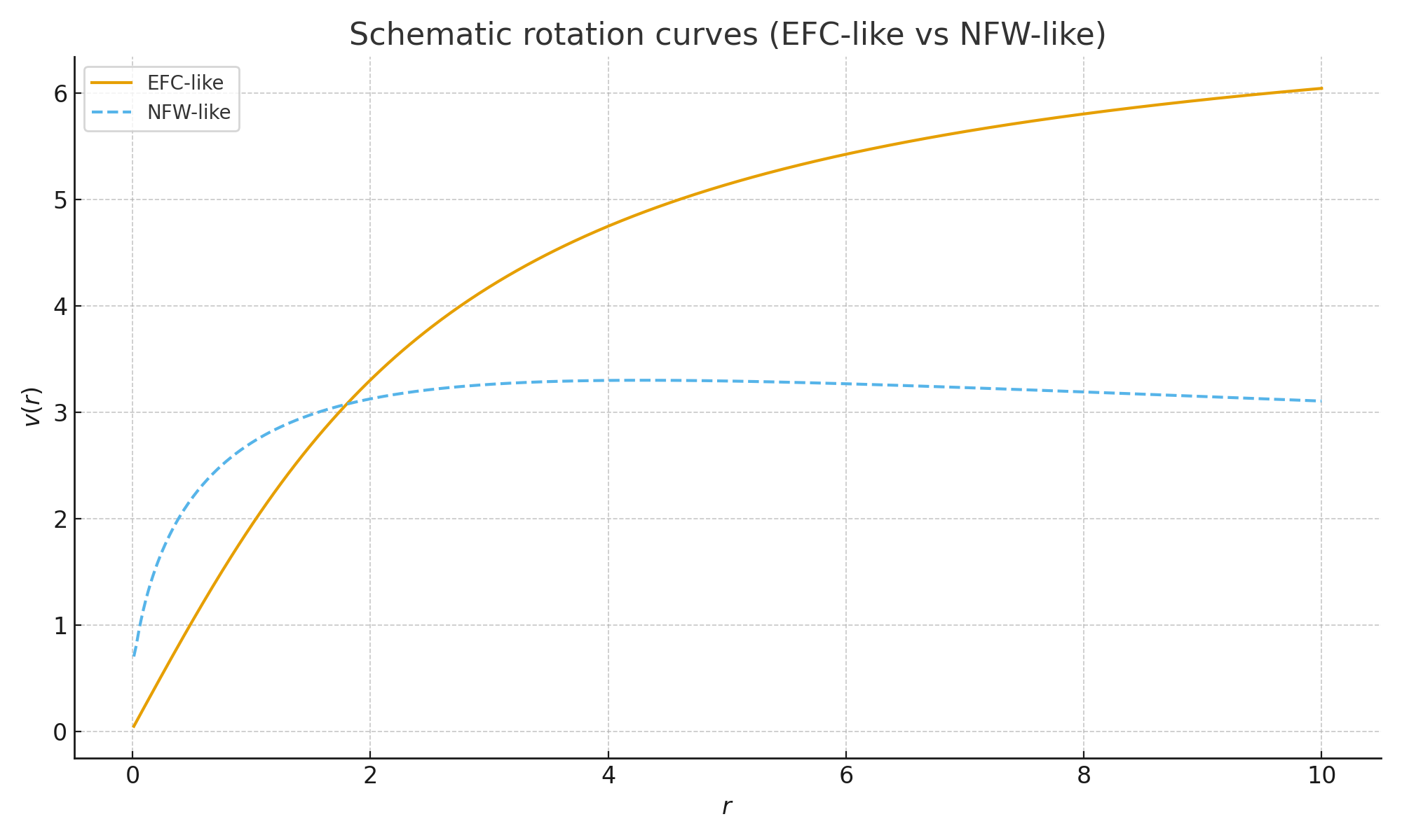
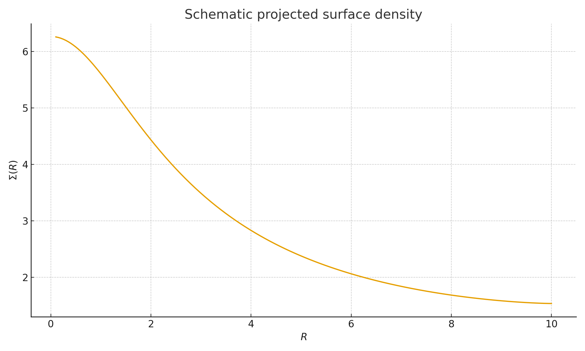
3.3 Rotation curves and projected density

Given a halo profile, EFC-D can be used to derive effective rotation curves and projected surface densities. Figure 4 shows a schematic comparison between an EFC-like rotation curve and an NFW-like reference. Figure 5 shows a corresponding schematic projected surface-density profile.

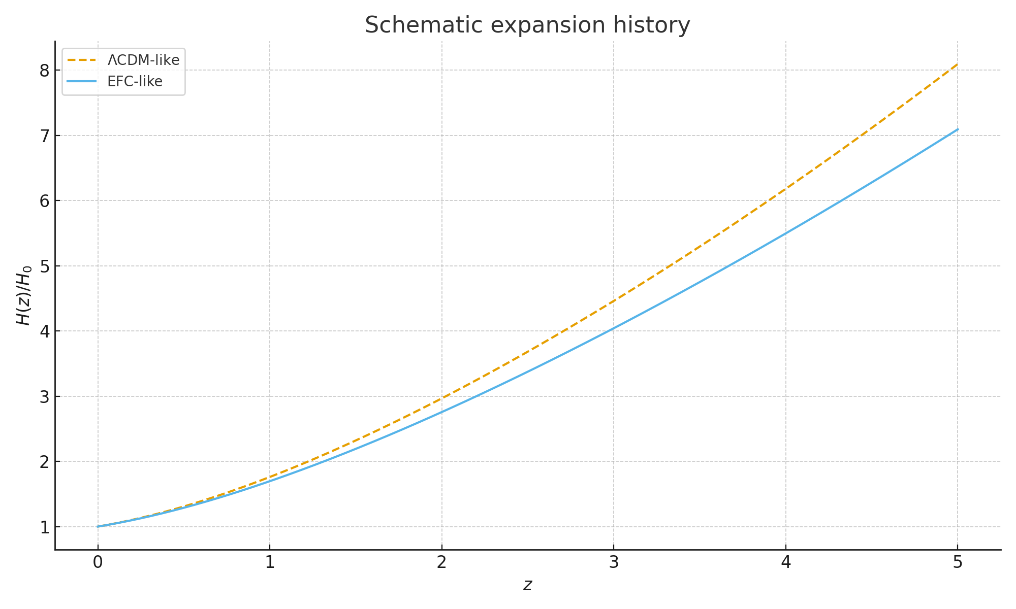
3.4 Expansion history and information capacity

EFC treats the effective expansion rate $H(z)$ as a derived quantity from flow and entropy, rather than a primary parameter. Figure 6 shows a schematic comparison between an EFC-like expansion history and a $\mathrm{\Lambda }$CDM-like reference. Figure 7 shows a simple information-capacity curve $I(S)\propto (1-S)$ at fixed density, relevant for EFC-C₀.

4. Part I — EFC-S: Structure / Halo Layer

4.1 S₀. Low-entropy anchors

EFC-S starts from the idea that structure forms around low-entropy anchors. These are local regions where matter and energy are concentrated in configurations that allow sustained energy flows.

Let $s(\mathbf{x})$ denote the entropy density at position $\mathbf{x}$. A low-entropy anchor is a region $\mathcal{A}$ such that:

where $⟨s⟩$ denotes a coarse-grained average. These anchors serve as seeds for halo formation and long-range correlations in the energy-flow field.

4.2 S₁. Halo Model of Entropy

In EFC-S, halos are not only mass overdensities, but also entropy-structured regions. A halo profile is described by both mass density and entropy:

where ${\rho }_h(r)$ is the radial mass density profile and $S_h(r)$ is a dimensionless entropy profile normalised to $[0,1]$. The combination $({\rho }_h(r),S_h(r))$ defines how effective a halo is as a driver for energy flows in EFC-D.

4.3 S₂. Radial profiles and halo classes

EFC-S allows families of halos parameterised by a small set of structural parameters (for example central density, scale radius and entropy core size). A simple example parametrisation is:

where $f$ and $g$ are chosen shape functions, $r_s$ is a mass scale radius, and $r_c$ is an entropy core radius. Different functional choices represent different halo classes in the EFC-S catalogue.

5. Part II — EFC-D: Energy-Flow Dynamics

5.1 D₀. Local energy-flow potential $E_f(\rho ,S)$

The local energy-flow potential $E_f$ depends on the mass density $\rho$ and entropy $S$. It captures how much structured energy-flow capacity a region has. At the baseline level:

High density with low entropy yields large $E_f$. High entropy suppresses $E_f$ even for dense regions.

5.2 D₀.2. Mass density

Mass density is defined in the usual way:

where $m$ is mass in a local region and $V$ is the associated volume.

5.3 D₁. Energy-flow rate and temporal evolution

The temporal change of the energy-flow potential defines an energy-flow rate:

where ${\mathrm{\nabla }}_t$ is the derivative along the chosen time parameter (cosmic time or another evolution parameter).

Using the definition of $E_f$ and applying the product rule, one obtains:

This separates contributions from density change and entropy change: a region can lose energy-flow potential by losing mass, by gaining entropy, or by both.

5.4 D₂. Spatial gradients and effective acceleration

Spatial gradients in $E_f$ define preferred directions of energy flow. At the field level:

which follows directly from the definition via the product rule.

At the level of an effective description, one can introduce an acceleration field $\mathbf{a}$ proportional to this gradient:

The minus sign indicates flow towards regions of lower effective potential, in analogy with standard potential theory, but here the potential is thermodynamic–structural rather than purely gravitational.

5.5 D₃. Expansion rate and background behaviour

On large scales, an effective expansion rate $H$ can be linked to coarse-grained energy-flow variables. A simple baseline relation uses the magnitude of $E_f$:

where $H_0$ is a reference scale and $F$ is a dimensionless function to be fixed by confrontation with data (e.g. supernovae, BAO, CMB). The important point for this master specification is not the exact form of $F$, but that $H$ is understood as a derived quantity from flow and entropy, not a primary parameter.

6. Part III — EFC-C₀: Entropy–Cognition Base Layer

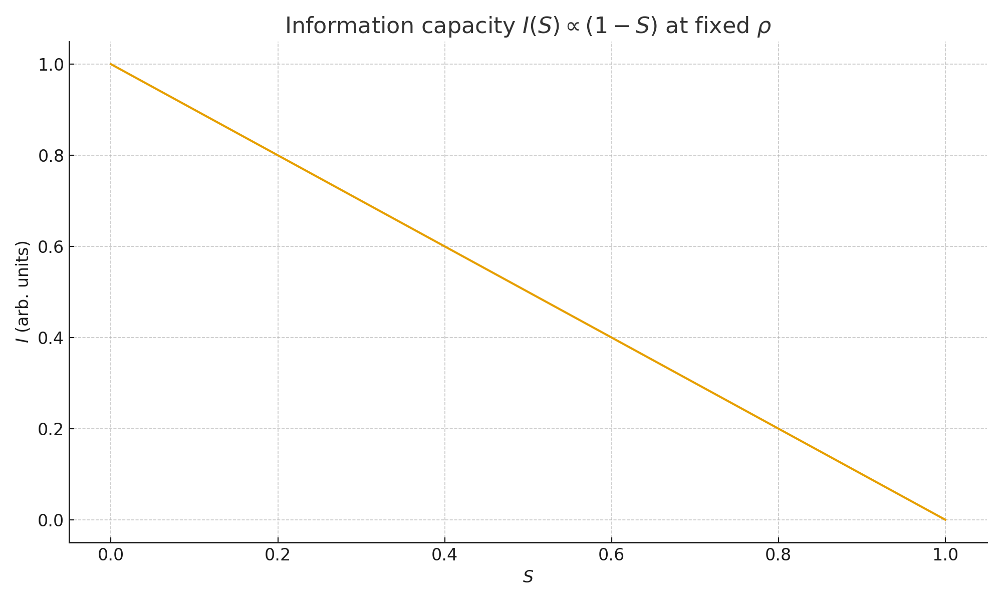
6.1 C₀. Entropy and information capacity

EFC-C₀ links thermodynamic entropy to potential for information processing. The goal is not a psychological model, but a base mapping between physical structure and abstract information capacity.

A local information capacity $I(\mathbf{x})$ is defined, at baseline, as:

This mirrors the structure of $E_f$, but $I$ is interpreted as a potential for storing and transforming information rather than driving motion directly.

6.2 C₁. Local cognitive load

For a coarse-grained region $\mathcal{R}$, define a total information capacity and a used fraction. The total capacity is:

A simple scalar cognitive-load variable $L$ can then be defined as:

where $I_{\text{used}}$ is the part of the available capacity that is currently engaged in maintaining or updating structure, patterns or internal models in the region.

6.3 C₂. Informational field coupling

EFC-C₀ treats information structures as coupled to the same energy-flow fields that drive dynamics in EFC-D. At a coarse-grained level, one can express this by letting $I$ respond to changes in $E_f$:

where:

• $\alpha$ scales how changes in energy-flow potential translate into increased or decreased information capacity,
• $\beta$ scales a dissipation term $D_I$ (for example diffusion, noise or degradation of structure).

This is a minimal base equation that later cognitive layers can extend.

7. Appendix: Symbols and Definitions

The table below summarises the main symbols used in this master specification.

8. How to Cite

9. References

This master specification can be combined with an external reference list (articles, datasets, code repositories). A fixed bibliography can be embedded in later versions.